Veridical Causal Inference/Propensity Score Tutorial (with R Code)
Summary
This is a tutorial for using propensity score methods for comparative effectiveness and causal inference research. The example uses medical claims data with R code provided at each step.
See the original paper: Ross, R.D., Shi, X., Caram, M.E.V. et al. Veridical causal inference using propensity score methods for comparative effectiveness research with medical claims. Health Serv Outcomes Res Method (2020). https://doi.org/10.1007/s10742-020-00222-8
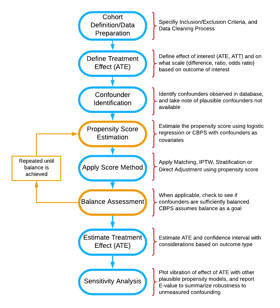
Flow diagram of stages of propensity score analysis. Gold pathway indicates steps done in iteration until acceptable balance is achieved.
Abstract
Medical insurance claims are becoming increasingly common data sources to answer a variety of questions in biomedical research. Although comprehensive in terms of longitudinal characterization of disease development and progression for a potentially large number of patients, population-based inference using these datasets require thoughtful modifications to sample selection and analytic strategies relative to other types of studies. Along with complex selection bias and missing data issues, claims-based studies are purely observational, which limits effective understanding and characterization of the treatment differences between groups being compared. All these issues contribute to a crisis in reproducibility and replication of comparative findings using medical claims. This paper offers practical guidance to the analytical process, demonstrates methods for estimating causal treatment effects with propensity score methods for several types of outcomes common to such studies, such as binary, count, time to event and longitudinally-varying measures, and also aims to increase transparency and reproducibility of reporting of results from these investigations. We provide an online version of the paper with readily implementable code for the entire analysis pipeline to serve as a guided tutorial for practitioners. The analytic pipeline is illustrated using a sub-cohort of patients with advanced prostate cancer from the large Clinformatics TM Data Mart Database (OptumInsight, Eden Prairie, Minnesota), consisting of 73 million distinct private payer insurees from 2001-2016.
Introduction and Background
Health service billing data can be used to answer many clinical and epidemiological questions using a large number of patients and has the potential to capture patterns in health care practice that take place in the real world (Sherman et al. 2016; Izurieta et al. 2019; Noe et al. 2019; Nidey et al. 2020; O’Neal et al. 2018). Such large datasets allow investigators to conduct scientific queries which may be difficult, if not practically impossible, to answer via a randomized clinical trial. For example, comparing multiple medications that are produced by different drug companies and with varying guidelines for their use for a disease may only be feasible in a real healthcare database (Desai et al. 2019; Jackevicius et al. 2016). Although these large data sources offer a wealth of information, there are many challenges and drawbacks, such as measured and unmeasured confounding, selection bias, heterogeneity, missing values, duplicate records and misclassification of disease and exposures. As regulatory agencies and pharmaceutical companies increasingly consider studying the real world evidence present in such databases, the importance of proper methodology, reporting, and reproducibility of the analysis for a broad audience of researchers is of necessity (FDA 2011; Motheral et al. 2003; Birnbaum et al. 1999; Johnson et al. 2009; Berger et al. 2017; Dickstein and Gehring, 2014; FDA 2018). We emulate newly introduced principles from the predictability, computability, and stability (PCS) framework for veridical data science (Yu et al. 2020) to examine comparative effectiveness research questions that administrative claims data can be used to address.
Healthcare claims data have been extensively criticized for its use in epidemiological research (Grimes 2010; Tyree et al. 2006). These types of data are wrinkled with issues such as outcome and covariate misclassification, missing data, and selection bias. For example, International Classification of Disease (ICD) codes are entered into administrative records by the care provider, often only for the purpose of billing, and thus certain diagnoses may be missed or overrepresented or may differ across providers (Tyree et al. 2006). There is no agreed upon algorithm for identifying widely used outcomes like Emergency Room visits, and thus many definitions across analysts and institutions are used (Venkatesh et al. 2017). While not as accurate as gold standard clinical trial data, these datasets are still valuable and sometimes the only source of real-world data for a wide variety of questions regarding drug utilization, effectiveness, and monitoring of adverse events (Hoover et al. 2011; Wilson and Bock 2012). Claims data have the benefit of reflecting how medications are actually being prescribed, and thus may provide a more accurate depiction of treatment benefit in practice or real-life evidence. Further, these datasets capture a more comprehensive picture of a patient’s encounters with the healthcare system than standard electronic medical record (EHR) data alone (Schneeweiss et al. 2005), going beyond just visits by adding procedures, tests, and pharmacy fills. With proper study design and methodological considerations, many of the common issues and concerns with claims data can be addressed (FDA 2011; Motheral et al. 2003; Birnbaum et al. 1999; Johnson et al. 2009; Berger et al. 2017; Dickstein and Gehring, 2014; FDA 2018),and these large databases of longitudinal information can provide insight into many research questions and be used to complement/supplement/emulate a clinical trial (Hernan and Robins, 2018).
While there are several approaches to handling confounding bias are available, propensity score-based methods are versatile in that they can be used for a variety of research questions and can be used for many different kinds of study designs and databases. Propensity score approaches also prevent p-hacking of a desired result in the outcome model (Braitman and Rosenbaum 2002). Thus, these methods have gained increasing popularity, especially for questions of comparative effectiveness in pharmacoepidemiologic and pharmacoeconomic research. With counterfactual thinking and causal inference gaining popularity in the statistical and epidemiological literature, principled use of propensity score based methods in observational databases have become more common.
A downside to this rise in popularity is that the assumptions and critical steps for the propensity score-based methods are often ignored or unreported. This lack of reporting hinders other researchers’ ability to replicate the findings. Many have noted common misuse or lack of reporting for propensity methods (Ali et al. 2015; Yao et al. 2017; Weitzen et al. 2004; Austin 2008; D’Ascenzo et al. 2012; Deb et al. 2016). Analysis questions arise, such as how the propensity score was calculated (logistic regression or otherwise), and even for many researchers who did describe such methods, sensitively analysis to the violation of assumptions or choice of the propensity score model were often not reported. Propensity score methods do not account for unmeasured confounding, and sensitivity analyses can provide the reader with crucial information on the robustness of the findings.
Some have offered valuable tutorials on propensity score estimation (Garrido et al. 2014; Austin 2011; Stuart et al. 2013; Brookhart et al. 2013). While these papers offer an elegant and lucid exposition of the underlying principles, and are extremely important contribution to the literature, these overviews do not provide the reader a complete practical guidance for every analysis step, or a detailed sensitivity analysis framework to understand the strength of evidence supporting the results when model assumptions change. Therefore, there is need for a usable, simple and comprehensive tutorial for all stages of analysis when characterizing a binary treatment effect on various outcome types using claims data, with accompanying annotated R software code for each step. This paper outlines the use of three primary propensity score-based methods: Spline Adjustment, Propensity Matching, and Inverse Probability of Treatment Weighting (IPTW) for comparing treatment effects with the goal of reducing bias due to confounding. The paper also details how to use each method to estimate average treatment effect for four common outcome types: 1) Binary, 2) Count, 3) Time to event, and 4) Longitudinally varying repeated measures. Finally, we conduct sensitivity analysis for two of the outcome types. The analytic pipeline is illustrated using a sub-cohort of patients with advanced prostate cancer from the large Clinformatics TM Data Mart Database (OptumInsight, Eden Prairie, Minnesota), consisting of 73 million distinct private payer insurees from 2001-2016.
Guideline for the Comparative Effectiveness Data Analysis Pipeline
Cohort Definition and Average Treatment Effect
The first stage of analysis is cohort definition. The STROBE checklist for cohort studies provides guidelines for defining a cohort and research question for analysis (von Elm et al. 2007). Once a cohort is defined, comparative effectiveness research for that cohort relies on the potential-outcomes framework, which as described by Rubin (1975 and 2005), involves comparison of potential outcomes on comparison of potential outcomes on the same (say \(i^{th}\)) individual. Define \(Y_{i}(0)\) as the potential outcome under the control treatment, and \(Y_{i}(1)\) as the potential outcome under the active treatment of interest. We wish to know the treatment effect for each individual, typically defined as \(Y_{i}(1) - Y_{i}(0)\), which cannot be estimated directly from the observed data because for each individual we observe either \(Y_{i}(0)\) or \(Y_{i}(1)\), but never both. If subject \(i\) actually received the active treatment, denoted by \(T_i=1\) then \(Y_{i}(1)\) is observed and \(Y_i =Y_{i}(1)\); otherwise, \(T_i=0\), and we observe \(Y_i=Y_{i}(0)\), under the stable unit treatment value assumption. Often, researchers are interested in how patients receiving a specific treatment compares to a comparison group within a larger population. We can define the average treatment effect (ATE) as \(E[Y_{i}(1) - Y_{i}(0)]\),which is the average treatment effect across the entire population.(Imbens 2004). In a randomized trial, we can estimate ATE as \(E[Y_{i}(1) - Y_{i}(0)] = E[Y_i|T_i=1] - E[Y_i|T_i=0]\) as randomization ensures that the treatment groups are balanced and hence \(E[Y_i(a)] = E[Y_i(a)|T_i=a] = E[Y_i|T_i=a]\) for all \(a = 0,1\) (Austin 2011b; Lunceford and Davidian 2017) ATE can be defined on different scales, such as a ratio \(\frac{E[Y_i|T_i=1]}{E[Y_i|T_i=0]}\) or odds ratio for binary outcomes \(\frac{E[Y_i|T_i=1]/(1-E[Y_i|T_i=1])}{E[Y_i|T_i=0]/(1-E[Y_i|T_i=0])}\) We can also define the average treatment effect on the treated (ATT) as \(E[Y_i(1)− Y_i(0)|T = 1]\) and the average treatment effect on the control (ATC) as \(E[Y_i(1)− Y_i(0)|T = 0]\) when a particular sub-population is of interest.
The standard method of estimating treatment effect for data from a randomized trial, or from observational data that is sufficiently balanced, is a general linear model with the treatment variable as the sole predictor:
\[ g(\mu_{i}) = \beta_{0} +\beta_{1}T_{i} \] where \(\mu_{i} = E[Y_{i}|T_i]\) and \(\beta_1\) is the parameter of interest for treatment comparison. In the simple linear regression case where \(g()\) is the identity function, \(\beta_1 = E[Y_i|T_i=1] - E[Y_i|T_i=0]\). When using claims data, the mechanism behind treatment assignment is not random, and thus the treatment populations may differ greatly. Therefore \(E[Y(1)|T = 1] \neq E [Y(1)]\) and \(E[Y(0)|T = 0] \neq E [Y(0)]\) in general (Austin 2011b). As a result, the estimate for \(\beta_1\) ATE will not confounding. Traditionally, confounders were adjusted for directly in the outcome model to obtain an estimate of ATE.
When confounders are present, a natural inclination would be to extend our outcome model to account for such confounders:
\[ g(\mu_{i}) = \beta_{0} +\beta_{1}T_{i} +\beta_{2}X_{2i} +...+\beta_{k}X_{ki} \]
However, \(\beta_1\) in the multivariate adjustment model generally does not estimate ATE even if we have the correct confounders and the model is correctly specified, particularly when \(g()\) is not a collapsible link function. One approach to estimate ATE is G-computation, which predicts the pair of potential outcomes for each individual (Robins 1986; Snowden et al. 2011). The accompanying standard error can be computed using sandwich estimation (Andersen 2019; Susanti et al. 2014). While a valid analytical approach, it may be difficult for the researcher to specify the outcome model, as there may be limited understanding of the relationship between the outcome and each covariate. The notion of the propensity score, a unidimensional construct, offers an alternative analytical approach that may be more suitable. The researcher may have more subject matter knowledge to construct a proper propensity score model, may want to avoid unconscious bias of demonstrating a desired causal effect in the outcome models by choosing confounders to adjust for, or use the propensity score simply as a dimension reduction technique.
Confounder Selection and Propensity Score Estimation
Proposed by Rosenbaum and Rubin (1983) the propensity score is \(e_{i}= Pr(T_{i} = 1| \boldsymbol{X}_{i} =x)\) . The score can be interpreted as the probability a subject receives treatment conditional on the covariates \(\boldsymbol{X}_{i}\). Rosenbaum and Rubin (1983) showed that conditional on the propensity score, an unbiased estimate of ATE can be obtained if the treatment is strongly ignorable. A treatment is strongly ignorable if two conditions are met: 1) \(0 <P(T_{i}=1|\boldsymbol{X}_{i})<1\) and \((Y_i(0),Y_i(1)) \perp \perp T_i|\boldsymbol{X}_i\) (Rosenbaum and Rubin 1983)
The second of these assumptions is the “no unmeasured confounders” assumption. Thus, a critical assumption for use of the propensity score is that all variables that affect the outcome and treatment assignment are measured. If all confounding variables are identified and included, and the model is correctly specified, this score achieves covariate balance between treatment and control groups. More formally, the correct \(e_i\) satisfies that \(T_i \perp \boldsymbol{X}_i |e_i,\) removing the effect of the confounders from the treatment effect when we condition on \(e_i\) alone. While logistic regression is commonly used to estimate this propensity score, researchers have expanded their attention beyond parametric models. Many have used machine learning methods such as boosted logistic regression, random forests, and neural networks (Lee et al. 2010; Setoguchi et al. 2008; Westreich 2010). Another method we highlight in this paper is the covariate balancing propensity score (CBPS) proposed by Imai and Ratkovic (2014).
Covariate Balancing Propensity Score (CBPS) is a generalized method of moments estimate that captures two characteristics of the propensity score, namely, as a covariate balancing score and as the conditional probability of treatment assignment (Imai and Ratkovic 2014). This method is a more automated form of propensity score construction, in that it calculates the propensity score with the exact balancing goal in mind. Thus, CBPS provides a balancing score for each subject that ensures all covariates included in the CBPS construction are balanced. Therefore, CBPS is an efficient alternative to propensity score estimation by a parametric model. We do note that if using another estimation technique, the ultimate goal of the propensity model is not to predict treatment assignment, but to reduce bias by balancing covariates (Wyss et al. 2014).
Still, the treatment effect estimation methods are sensitive to misspecification of the propensity score model, and thus the variables and their functional forms used in this model can affect the estimation of average treatment effect. Many suggest including all variables at all associated with the outcome, while excluding those only associated with the treatment of interest, based on subject-matter knowledge.[33,48,49,50,51] Vanderweele[52] provides a comprehensive general guide to confounder selection in observational studies. The sensitivity analysis can show how estimates can change under many plausible propensity score models.
Application of the Propensity Score
Once the propensity score is constructed, there are four basic ways to use the score in treatment effect estimation: 1) Stratification based on the propensity score, 2) Direct covariate adjustment using propensity score as a covariate in the outcome model, 3) Matching treatments and controls based on the propensity score (PM), and 4) Inverse probability treatment weighting on the propensity score (IPTW). Stratification ranks subjects by the estimated propensity score and splits them into mutually exclusive stratum (say, deciles). The treatment effect in each stratum (decile) can then be estimated and pooled to obtain an overall treatment effect.[53] We will not discuss stratification at length in the main paper as it is used less commonly,[54,55] but we do provide a quickstart. The rest of this tutorial will focus on the three routinely used methods: Spline Adjustment, Propensity Matching, and IPTW.
Spline Adjustment
Once the propensity score is constructed, there are four basic ways to use the score in treatment effect estimation: 1) Stratification based on the propensity score, 2) Direct covariate adjustment using propensity score as a covariate in the outcome model, 3) Matching treatments and controls based on the propensity score (PM), and 4) Inverse probability treatment weighting on the propensity score (IPTW). Stratification ranks subjects by the estimated propensity score and splits them into mutually exclusive groups to obtain an overall treatment effect (Rosenbaum and Rubin 1984). We will not discuss stratification at length in the main paper as it is used less commonly (Austin et al. 2007; Austin 2009b), but the online materials provide further information. The rest of this paper will focus on the three routinely used methods: Spline Adjustment, Propensity Matching, and IPTW.
Propensity Matching
Matching observations based on the propensity score to estimate ATT and is based on a measure of distance (Stuart et al. 2010; Rosenbaum and Rubin 1985a). Stuart et al. (2010) provide a comprehensive overview of the various matching methods available. In practice, it is common to do 1:k matching, where k is the specified number of controls. With a defined distance, called a caliper, all potential matches within the distance up to k will be matched. This allows for maximal efficiency of data while still reducing bias since all close matches are kept. There is little guidance on what caliper a researcher should specify; however, Austin (2011a) suggests a caliper of 0.2 standard deviations of the logit of the propensity score as a default choice that works well across scenarios. Matching typically estimates the ATT, though some packages and techniques can estimate ATE (Stuart et al. 2010).
Inverse Probability of Treatment Weighting (IPTW)
The next method we consider is the inverse probability of treatment (IPTW) proposed by Rosenbaum (1987) We can calculate the IPTW \(v_i\) as \[ v_{i} = \dfrac{T_{i}}{\hat{e}_{i}} + \dfrac{(1-T_{i})}{(1-\hat{e}_{i})} \] where \(\hat{e_i}\) is the estimated propensity score. These weights can be very unstable for extreme values of \(\hat{e_i}\), These weights can be very unstable for extreme values of ^(e_i ), so trimming (sometimes called truncating) these values away from the extreme is often practiced (Rosenbaum 1987; Lee et al. 2011). The construction of weights used here estimates ATE, and different constructions can be used for ATT and other effect estimates of interest (Lee et al. 2011).
Balance Assessment
It is good practice to check if the chosen propensity method achieved its goal of balancing the covariates. While there are several balance diagnostics a common balance diagnostic originally proposed by Rosenbaum and Rubin (1985b) is the standardized difference (or standardized bias) for \(1:1\) matching, defined as \[ \frac{\bar{x}_{t} - \bar{x}_{c}}{s_{p}} \] This is the difference in mean value of the covariate in the treatment group vs. the control group, adjusting for variability, where \(s_{p}\) is the pooled standard deviation defined as \(s_{p}=\sqrt{\frac{s_{t}^2 +s_{c}^2}{2}}\).(Austin 2009a; Normand et al. 2001). This value is calculated for each covariate, with values closer to zero indicating better mean balance and potentially less bias. The measure can be calculated for both continuous and categorical indicator variables (Yao et al. 2017; Normand et al. 2001). A lack of balance indicates that the propensity model may be incorrect, or that a different method should be used. There is no generally accepted threshold, although some suggest that the standardized difference should not be greater than \(0.1\).(Austin 2008b; Austin 2009a; Normand et al. 2001). We can modify this difference calculation for a different ration of matching, say \(1:k\), using weights (Joffe et all. 2004; Morgan and Todd 2008; Austin 2008b). The weighted mean is defined as \(\bar{x}_{w} = \frac{\sum w_{i}x_{i}}{\sum w_i}\) and the weighted standard deviaion is \[ s_{w} = \sqrt{\dfrac{\sum w_{i}(x_i - \bar{x}_{w})^2}{\frac{\sum w_{i}}{(\sum w_i)^2 - \sum {w_i}^2}}} \] where \(w_i\) is the weight for subject \(i\). For \(1:1\) matching, all observations have equal weight. If \(1:k\) matching is used, observations in the control treatment group have \(1/k\) weights and treated observations have weights \(1\). For IPTW, the calculated weights can be used, so \(v_i = w_i\) for each observation (Morgan and Todd 2008; Austin 2008b). If sufficient balance is not achieved, the process of propensity score construction and balance assessment is repeated, by changing the functional form of the propensity model. The researcher can repeat this process until balance is achieved to a desired level. Experimenting with the model specification at this stage is preferable to post-hoc modification of the outcome model with ATE as a desired target, especially in terms of reproducibility of results.
Treatment Effect Estimation
Once sufficient balance has been achieved, one can estimate the average treatment effect using a general outcome model \[ g(\mu_{i}) = \beta_{0} +\beta_{1}T_{i} \]
This model can be used directly on the matched dataset if 1:1 matching is used. If 1:k matching or IPTW is used, the constructed weights need to be used as well. Weights can be incorporated in the same fashion as weights from a survey design, using robust standard error estimation to account for error in weight estimation (Lee et al. 2001; Morgan and Todd 2008). For the spline adjustment model, ATE is estimated by G-computation with direct variance calculation via M-estimation (Stefanski and Boos, 2002). Once an estimate is obtained, it is often useful to run a sensitivity analysis to see how the estimate may change under different model specifications and understand how sensitive the result is to some unmeasured confounder.
Sensitivity Analysis
For the sensitivity analysis, we adapt a visualization tool of capturing vibration of effects from Patel et al. (2015) to a universe of potential propensity score models. This visualization tool allows the researcher to see the results of many possible models at once, providing an overall understanding of the treatment effect estimate’s robustness to changing model specifications with the observed set of measured confounders. To summarize sensitivity to an unobserved/unmeasured confounder, we calculate the estimate’s E-value (Van Der Weele and Ding 2017). The E-value captures the minimum value of the association parameter that an unobserved confounder must have with both the treatment and the outcome of interest to nullify the result regarding the treatment effect on the outcome. Put more simply, the E-value tells us how strong an unmeasured confounder must be to explain away a significant treatment effect.
Data for Illustrated Example
Cohort Definition and Average Treatment Effect
Many patients with advanced prostate cancer will receive a number of different therapies sequentially to try to control the disease and symptoms. The three different types of outcomes that we consider are based on what clinicians are typically interested in. Patients may have varying degrees of responsiveness and tolerance to different therapies during the period of treatment. For example, some patients who experience pain from their cancer will have pain relief after starting a treatment and thus require less opiates to manage their cancer. On the other hand, some patients will have poor tolerance of specific therapies and may experience exacerbation or development of comorbid conditions and seek emergency critical care. It is also important to note that a treatment is typically only continued for as long as it is effectively controlling the disease or symptom. Thus, the longer a patient is on a treatment, presumably the longer the duration of effective disease control on that treatment.
Cohort Definition and Data Preparation
The cohort was defined as men who received treatment for advanced prostate cancer at any time during January 2010 through June 2016, based on receiving one of four primary medications (abiraterone, enzalutamide, sipuleucel-T, docetaxel) known to have a survival benefit in men with advanced prostate cancer. Data were from the Clinformatics TM Data Mart Insurance Claims Database. The initial cohort included any patient over the age of 18 with a diagnosis of malignant neoplasm of the prostate, coded as “185” in ICD-9 and “C61” in ICD-10, and were continuously enrolled in the plan for at least 180 days before the first medication claim.
Treatments: We are interested in comparing first-line therapies. First-line treatment was defined as the first medication given of the four focus medications. We then categorized oral therapies as abiraterone or enzalutamide. Thus, there are three final first-line treatment groups: 1) Immunotherapy, 2) Oral Therapy, and 3) Chemotherapy. We compared immunotherapy to oral therapy and compared immunotherapy to chemotherapy in two separate analyses. We chose immunotherapy as the reference group for both analyses. The remainder of this example will only discuss the oral therapy comparison, as all methods are directly translatable, and we report all results for both analyses in the tables.
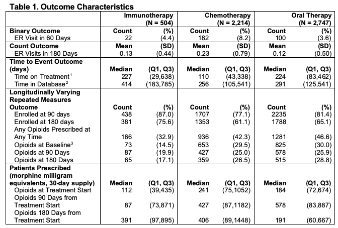
Binary and Count Outcomes : We defined the binary outcome to be whether the patient had any emergency room (ER) visit within 60 days of the first pharmacy claim of the focus medications. ER visits were identified using the provider definition, Current Procedural Technology (CPT) codes 99281-99285, and the facility definition, which is revenue center codes 0450-0459, 098 (Vankatesh et al. 2017; CMS 2020a, CMS 2020b). ATE is defined on the odds ratio scale. Using the previously defined ER visits, we counted the number of ER visits each patient had within 180 days from the first pharmacy claim as a count outcome. ATE is defined on the rate ratio scale.
Time to Event Outcome: Time on treatment, the time to event outcome, was defined as the time from start of first medication to the last claim of any of the four focus medications, thus the event is stopping all focus treatment permanently. ATE is defined in terms of Restricted Mean Survival Time (RMST) (Royston et al. 2013; Andersen 2010) within a five year follow-up window. We can calculate RMST, denoted μ_τ, as the area under the curve of the survival function: \[ \mu_\tau = \int_{0}^{\tau} S(t) dt \] where \(S(t)\) is the survival function, and \(\tau\) is the parameter for restricted the follow up time. We can then define our ATE estimate as \(\mu_{\tau1} - \mu_{\tau0}\), or the difference in RMST between the treatment groups being compared.
Longitudinally Varying Outcome: For the longitudinally varying outcome, we used opioid usage over time, calculated using prescription drug pharmacy claims. Common opioid drug types were identified and were converted into morphine milligram equivalents (MME) according to the Center for Disease Control conversion factors (CDC 2020). The average daily MME supply prescribed was calculated in 30-day periods, starting with the 30 days before the first-line of treatment, which was used as a baseline, and continuing at 30-day intervals for the duration of claims data available. ATE is defined as the mean difference in opioids prescribed at three specified time points: treatment start, 3 months after treatment start, and 6 months after treatment start. We can model the quantity of opioids prescribed in MME \(Y_{ij}\) at the 30 day period \(t_j\) for each individual \(i\) as:
\[ Y_{ij} = \beta_{0} + b_{0i} + \beta_{1}T_{i} + S(t_{j}) +S(t_{j})T_{i} +\epsilon_{ij} \]
where \(j=1,..,n_{i}\), \(n_{i} \in \{1,2,3,4,5,6,7\}\), \(b_{0} \sim N(0,\tau^{2})\) and \(\epsilon_{i} \sim MVN_{n_{i}}(0,\sigma^{2}I_{n_{i}})\). \(S(t_{ij})\) is specified as a penalized regression spline with 3 degrees of freedom, allowing more flexible smooths for modeling the prescribing trend over time. An important note when using IPTW and CBPS is that we are only weighting on the initial treatment, so at other time points the weights may bias the results. Any inferences using the full time period will be heavily biased by changing therapy or require advanced methods to handle switching treatments, such as marginal structure models (Cole and Hernan 2008).
Propensity Score Analysis Pipeline
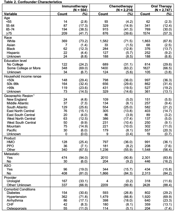
Confounders: Potential confounders were identified using previous research to identify factors associated with both treatment and outcomes (Hoffman et al. 2011; Ward et al. 2004; Caram et al. 2019a; Barocas and Penson 2010; Caram et al. 2019b). These include age, race, sociodemographic variables and comorbid conditions from Elixhauser Comorbidity Index and Clinical Classification Software (CMS 2020a, CMS 2020b), all shown in Table 2. From the table, we can see differences across treatments groups, especially age, geographic region, and provider type. These variables may inform treatment assignment and as such should be considered as potential confounders.
Propensity Score Estimation
We can construct a model for treatment assignment, \(T_{i}=0\) if immunotherapy was given and \(T_{i}=1\) if oral therapy was given using logistic regression, and the CBPS method. From the regression results, we can calculate the estimated propensity score for each subject. It is often helpful to plot the distribution of propensity scores between the two groups of comparison, as shown below, especially if matching subjects based on the propensity score. If there is little or no overlap in the distributions, many subjects will not be included in analysis as matches will not be found. The propensity score constructed from the CBPS approach was implemented through the R package CBPS. (Imai and Ratkovic 2013). The weights from this propensity score were used in the outcome models similar to the inverse probability weights.
#create subsets for treating oral therapy and immunotherapy separately
oral<-firstline_single[firstline_single$pae<99,]
oral$treatment<-oral$pae

#restrict to subjects that were enrolled for at least 60 days for our 60 day outcome
oral60<-oral %>%
  filter(enrolltime >=60)


#calculate propensity score using logistic regression model
prop_model <-glm(treatment~agecat+racecat+educat+housecat+Division+Product+met+Aso+diabetes+
  hypertension+CHF+osteoporosis+arrythmia+uro,data=oral60,family=binomial(link="logit"))

#save predicted scores to dataset
oral60$pr_score <-predict(prop_model,type="response")
It often helps to plot the distribution of the propensity scores by the treatment. We wish to see some overlap in the distributions and not a perfect separation.
library(ggplot2)
library(ggpubr)
#this plots the distribution of our estimated propensity scores
g<- ggplot(oral60,aes(x = pr_score, color=Treatment,fill=Treatment)) +
  geom_density(alpha=.47) +
  xlab("Estimated Probability of Recieving Oral Therapy") +
  ylab ("Density") +theme_minimal()+ theme(
                           axis.ticks.y=element_blank(),
                         panel.grid.minor=element_blank(),
                         legend.title=element_blank(),
                         text = element_text(size=16),
                         axis.title.x =element_text(hjust = 0.2,size=16))
ggpar(g,palette="nejm")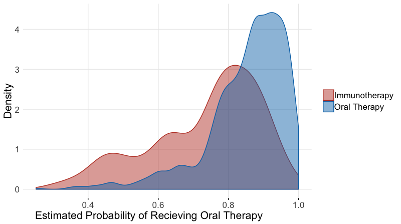
Now we calculate the scores using CBPS
library(CBPS)
#calculate weights using CBPS package and function
cbpsoral <-CBPS(treatment~agecat+racecat+educat+housecat+Division+Product+met+Aso+diabetes+
  hypertension+CHF+osteoporosis+arrythmia+uro,data=oral60,standardize=FALSE,method="exact",ATT=1)
## [1] "Finding ATT with T=1 as the treatment. Set ATT=2 to find ATT with T=0 as the treatment"oral60$cbps <-cbpsoral$weightsPropensity Score Matching
To create a matched dataset, we used the R package Matchit. We defined our distance with logistic regression using the “nearest neighbor” method select matches within a defined caliper distance of 0.2 standard deviations of the logit propensity score, with a variable matching ratio of 1:4 within the defined caliper, without replacement. These matching specifications were chosen to ensure maximal efficiency of this data. By using variable matching, we allow multiple matches for a subject in the control group if several in the treatment group have close propensity scores by our defined distance measure. This allows us to retain more subjects in our analysis dataset than a standard 1:1 ration. The caliper was decided using an iterative process, where several calipers were assessed and the one providing the highest quality matched sample was kept, based on the standardized differences across the covariates.
#create matched dataset based on same propensity model
#here we switched the outcome, as matchit requires the larger group to be the reference if variable ratio is being used
#We are capturing up to 4 oral therapy matches for every sipuleucel-T subject
matched <- matchit((1-treatment)~agecat+racecat+educat+housecat+Division+Product+met+Aso+diabetes+
  hypertension+CHF+osteoporosis+arrythmia+uro,data =oral60, method = "nearest",caliper=.2,ratio=4)

#looked at characteristics of matched object
matched_sum<-summary(matched)
matched_sum$nn
## Control Treated
## All 2363 471
## Matched 1421 455
## Unmatched 942 16
## Discarded 0 0#save matched dataset
matched_oral <- match.data(matched)Inverse Probability Treatment Weighting
Weights were created from both the logistic regression and CBPS estimated propensity scores using the formula described above. Some weights were unstable, so propensity scores greater that \(0.99\) were trimmed to \(0.99\), and scores below \(0.01\) were trimmed to \(0.01\). Trimmed weights were used for analysis.
#trim extreme values for stability
oral60$pr_score_trim <-if_else(oral60$pr_score<.01,.01,oral60$pr_score)

#now for the high values, retaining the lower trims
oral60$pr_score_trim <-if_else(oral60$pr_score>.99,.99,oral60$pr_score_trim)

#alternatively, a nested if_else can do the job in one line
#oral60$pr_score_trim <-if_else(oral60$pr_score<.01,.01,                       if_else(oral60$pr_score>.99,.99,oral60$pr_score))

#save the inverse weights from the propensity score
oral60$IPTW <-oral60$treatment/oral60$pr_score_trim + (1-oral60$treatment)/(1-oral60$pr_score_trim)
Stratification
Here we provide a brief example of using propensity score stratification. Once the propensity score is calculated, the data can be stratified based on specified quantiles of the propensity score distribution. Researchers suggest 5 strata is often sufficient. Balance diagnostics can then be checked within each strata. If sufficient balance is achieved, estimates from each strata can be estimated and then combined as if a meta-analysis, weighting each group inversely by the variance. R package PSAgraphics is a quick way to check balance, and meta can be used to obtain final estimate
library(gtools)

oral60$pr_cut <- as.numeric(factor(quantcut(oral60$pr_score_trim,q=5),labels=c(1,2,3,4,5)))
table(oral60$treatment,oral60$pr_cut)
##
## 1 2 3 4 5
## 0 210 116 75 54 16
## 1 357 454 488 513 551library(PSAgraphics)
model_mat <-model.matrix(~ +agecat+racecat+educat+housecat+Division+Product+met+Aso+diabetes+
hypertension+CHF+osteoporosis+arrythmia+uro -1,oral60)
cv.bal.psa(covariates = model_mat, treatment = oral60$treatment, propensity = oral60$pr_score,strata=5)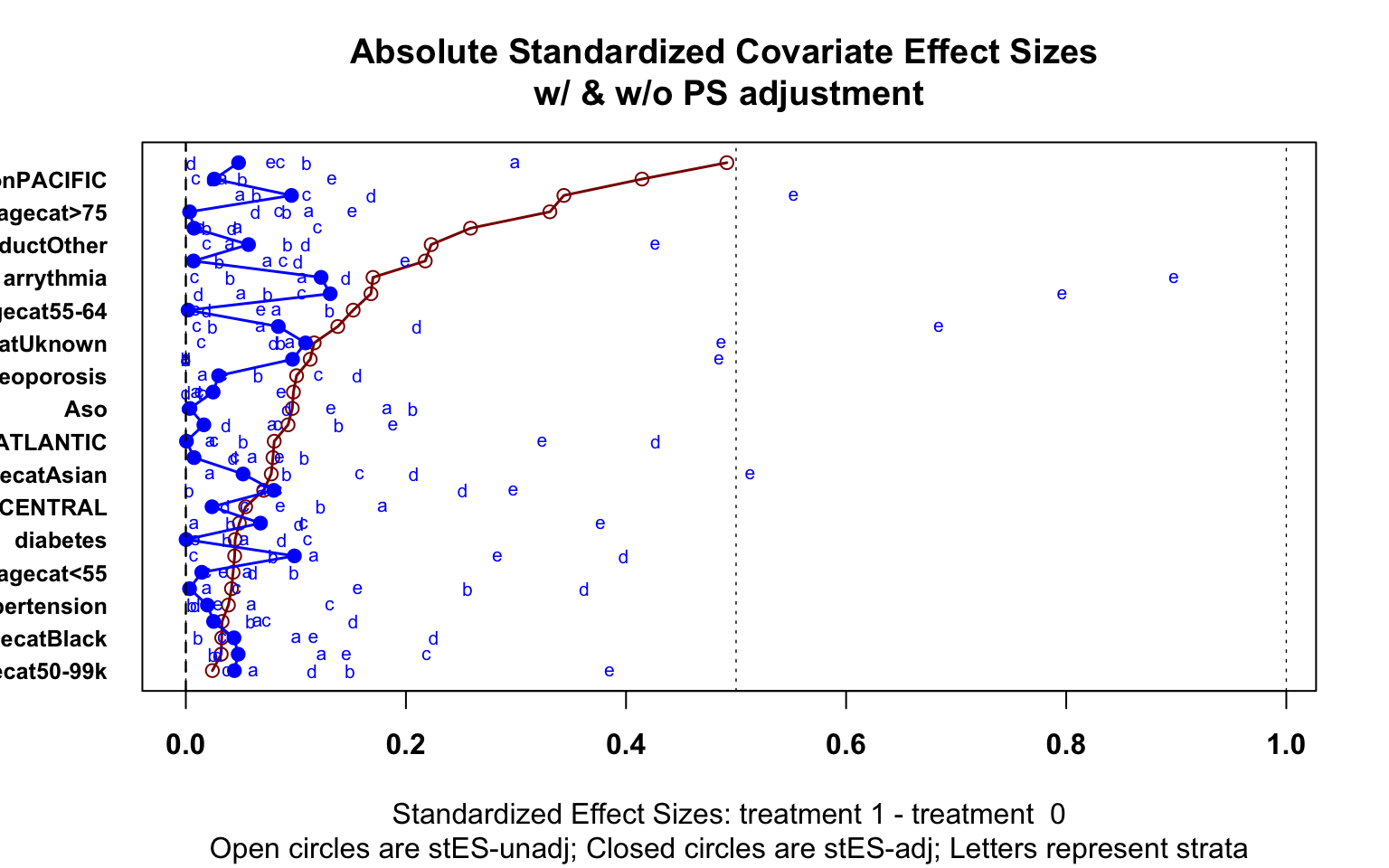
library(meta)

cells <-table(oral60$er60,oral60$treatment,oral60$pr_cut)

ai <- cells[1,1,]
bi <- cells[1,2,]
ci <- cells[2,1,]
di <- cells[2,2,]

meta <-metabin(event.e = di, n.e = ci + di,
                      event.c = bi, n.c = bi + ai,
                      sm = "OR", studlab = paste("propensity", c(1:5), sep = ""),
                      method="MH",
                      label.e="Oral Therapy", label.c="Immunotherapy", outclab = "ER Visit",
                      comb.fixed = TRUE, comb.random = FALSE)

forest.meta(meta)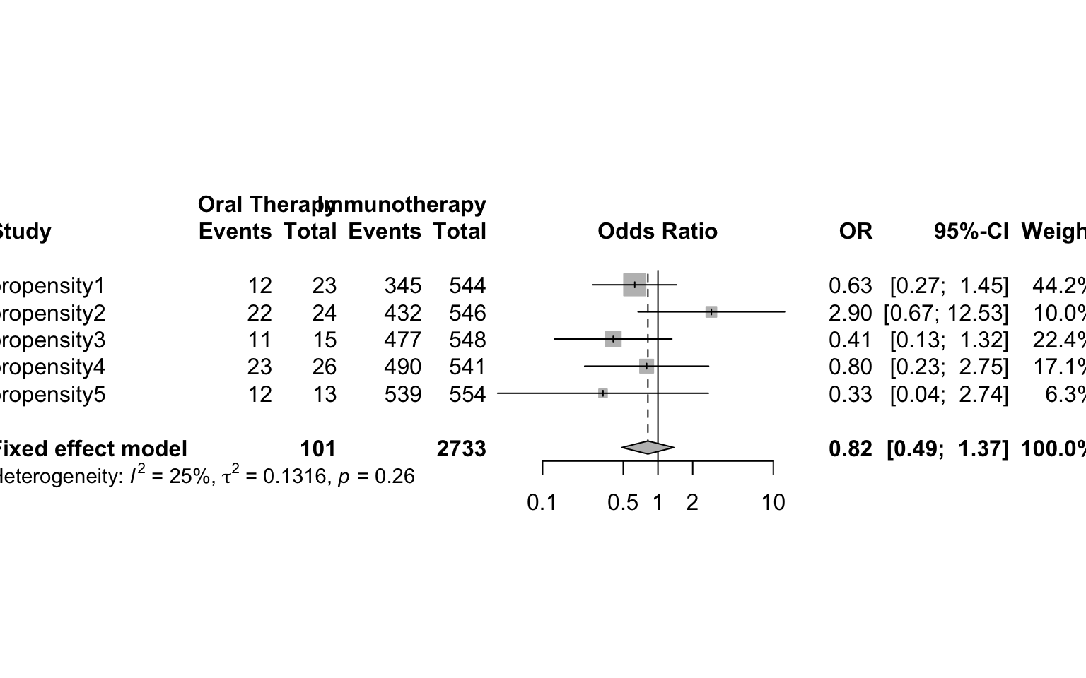
Assessment of Covariate Balance
Each method can be assessed for successful reduction in standardized difference for the analysis sample. Figure 3 shows a plot of the standardized difference of the covariates between the immunotherapy group, and oral therapy group for CBPS, IPTW and propensity matching methods. We can see that the inverse weighted data and the matched sample reduced the standardized difference for many covariates, even if perfect balance was not achieved. Unsurprisingly, the CBPS weights have very low/no bias, as the weights are constructed to achieve this goal of exact matching. With balance among the covariates achieved, we can now begin treatment effect estimation.
###################figure
#for forest plot to check the standardized differences
#create dummy variables for the many categorical variables
model_mat <-model.matrix(~treatment +agecat+racecat+educat+housecat+Division+Product+met+Aso+diabetes+
  hypertension+CHF+osteoporosis+arrythmia+uro -1,oral)

model_mat <-data.frame(model_mat)


#calculate means and standard deviations of each variable by group
fullsamp_means <-model_mat %>%
  group_by(treatment) %>%
  summarise_all(funs(mean))

fullsamp_var <-model_mat %>%
    group_by(treatment) %>%
  summarise_all(funs(sd))

fullsamp_std <-data.frame(t(fullsamp_var))
fullsamp_std$pooled <- sqrt(((fullsamp_std[,1])^2 + (fullsamp_std[,2])^2)/2)

fullsamp<-data.frame(t(fullsamp_means),fullsamp_std$pooled)

#calculate the standardized difference of the observed sample
colnames(fullsamp)<-c("sip_mean","oral_mean","sd")
fullsamp$bias <-(as.numeric(as.character(fullsamp$sip_mean))-as.numeric(as.character(fullsamp$oral_mean)))/as.numeric(as.character(fullsamp$sd))
fullsamp$group <-rep("Observed",nrow(fullsamp))
fullsamp$label <-rownames(fullsamp)


######matched group
#same calculations, now for the saved matched dataset
model_mat <-model.matrix(~treatment +agecat+racecat+educat+housecat+Division+Product+met+Aso+diabetes+
  hypertension+CHF+osteoporosis+arrythmia+uro+weights -1,matched_oral)

model_mat <-data.frame(model_mat)

matched_means <-model_mat %>%
  group_by(treatment) %>%
  summarise_all(funs(weighted.mean(., weights)))

matched_var <-model_mat %>%
  group_by(treatment) %>%
  summarise_all(funs(sqrt(sum(weights*(.-weighted.mean(., weights))^2/((n()-1)/n()*sum(weights))))))

matched_std <-data.frame(t(matched_var))
matched_std$pooled <- sqrt(((matched_std[,1])^2 + (matched_std[,2])^2)/2)

matched<-data.frame(t(matched_means),matched_std$pooled)

#remove the last row of our dataframe which contains the weights
matched<-matched[-nrow(matched),]

colnames(matched)<-c("sip_mean","oral_mean","sd")
matched$bias <-(as.numeric(as.character(matched$sip_mean))-as.numeric(as.character(matched$oral_mean)))/as.numeric(as.character(matched$sd))
matched$group <-rep("Matched",nrow(matched))
matched$label <-rownames(matched)


#####IPTW Group
#same calcuation using the inverse probability weights
model_mat <-model.matrix(~treatment +agecat+racecat+educat+housecat+Division+Product+met+Aso+diabetes+
  hypertension+CHF+osteoporosis+arrythmia+uro+IPTW -1,oral60)

model_mat <-data.frame(model_mat)
#model_mat$treatment <-as.factor(model_mat$treatment)


weighted_means <-model_mat %>%
  group_by(treatment) %>%
  summarise_all(funs(weighted.mean(., IPTW)))

weighted_var <-model_mat %>%
  group_by(treatment) %>%
  summarise_all(funs(sqrt(sum(IPTW*(.-weighted.mean(., IPTW))^2/((n()-1)/n()*sum(IPTW))))))

weighted_std <-data.frame(t(weighted_var))
weighted_std$pooled <- sqrt(((weighted_std[,1])^2 + (weighted_std[,2])^2)/2)

weighted<-data.frame(t(weighted_means),weighted_std$pooled)

#remove the last row of the dataframe
weighted<-weighted[-nrow(weighted),]

colnames(weighted)<-c("sip_mean","oral_mean","sd")
weighted$bias <-(as.numeric(as.character(weighted$sip_mean))-as.numeric(as.character(weighted$oral_mean)))/as.numeric(as.character(weighted$sd))
weighted$group <-rep("Logistic IPTW",nrow(weighted))
weighted$label <-rownames(weighted)


#####CBPS Group
#same calculations using the covariate balance propensity score weights

model_mat <-model.matrix(~treatment +agecat+racecat+educat+housecat+Division+Product+met+Aso+diabetes+
  hypertension+CHF+osteoporosis+arrythmia+uro+cbps -1,oral60)

model_mat <-data.frame(model_mat)
#model_mat$treatment <-as.factor(model_mat$treatment)


cbps_means <-model_mat %>%
  group_by(treatment) %>%
  summarise_all(funs(weighted.mean(., cbps)))

cbps_var <-model_mat %>%
  group_by(treatment) %>%
  summarise_all(funs(sqrt(sum(cbps*(.-weighted.mean(., cbps))^2/((n()-1)/n()*sum(cbps))))))

cbps_std <-data.frame(t(cbps_var))
cbps_std$pooled <- sqrt(((cbps_std[,1])^2 + (cbps_std[,2])^2)/2)

balanced<-data.frame(t(cbps_means),cbps_std$pooled)

#remove last row containing weights
balanced<-balanced[-nrow(balanced),]

colnames(balanced)<-c("sip_mean","oral_mean","sd")
balanced$bias <-(as.numeric(as.character(balanced$sip_mean))-
                   as.numeric(as.character(balanced$oral_mean)))/as.numeric(as.character(balanced$sd))
balanced$group <-rep("CBPS IPTW",nrow(balanced))
balanced$label <-rownames(balanced)


#construct plot data frame from all calculations
plot_data <-rbind(fullsamp,matched,weighted,balanced)


#change label names for presentation purposes
plot_data$label <-c("Sip","Age: <55","Age: 55-64","Age: 65-74","Age: >74","Race: Asian","Race: Black","Race: Hispanic", "Race: Unknown","Educaton: Some College","Education: Unknown","Income: 50-99K", "Income: >99k", "Income: Unknown","Region: East South Central","Region: Middle Atlantic", "Region: Mountain","Region: New England","Region: Pacific","Region: South Atlantic","Region: Unknown","Region: West North Central","Region: West South Central","Product: Other","Product: PPO","Metastatic: Yes","ASO: Yes","Diabetes: Yes","Hypertension: Yes","CHF: Yes","Osteoporosis: Yes","Arrhythmia: Yes","Provider: Urologist")


#remove row where bias is infinite because there are no subjects in control group
'%!in%' <- function(x,y)!('%in%'(x,y))
plot_data <-plot_data %>%
  filter(label %!in% c("Sip","Region: Unknown","treatment"))


library(ggplot2)
library(ggpubr)
library(ggsci)
#visual inspect covariate balance using ggplot
fp <- ggplot(data =plot_data,aes(x=label, y=bias,color=group,shape=group)) +
  scale_shape_manual(values=c(20,18,17,15))+
    geom_hline(yintercept=-0.1, lty=3,size=0.7) +
  geom_hline(yintercept=0.1,lty=3,size=0.7) + #these lines indicate the thresholds for high differences

  geom_point(size=5) +
  geom_hline(yintercept=0, lty=2) +  # add a dotted line at x=1 after flip
  coord_flip() +  # flip coordinates (puts labels on y axis)
  xlab("Variable") + ylab("Standardized Difference") +
  theme_minimal()+ theme(
                           axis.ticks.y=element_blank(),
                         panel.grid.minor=element_blank(),
                         legend.title=element_blank(),
                         text = element_text(size=16),
                         axis.title.x =element_text(hjust = 0.2,size=16)) #additional aesthetic options
ggpar(fp,palette="nejm")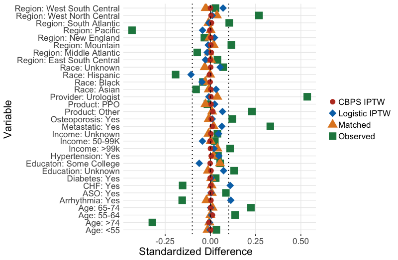
Treatment Effect Estimation
Binary Outcome: Visit to the Emergency Room (ER) in 60 days
First we fit the marginal, unadjusted model. This is not a causal estimate, as we saw above that the potential confounders are unbalanced.
#model the unadjusted treatment effect
mod_unad <-glm(er60~treatment,data=oral60,family=binomial(link=logit))
#summarize model results
#summary(mod_unad)

#now see odds ratio and confidence interval after expoentiation
#exp_out is a manually defined function - see tab for function code
exp_out(mod_unad)
## OR Lower Upper
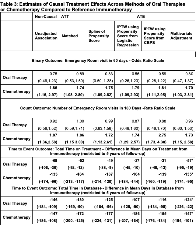
## treatment 0.75 0.46 1.23After running this model, we get an estimate of 0.75 (0.46,1.23), also reported in Table 3. This odds ratio indicates that patients treated with oral therapy first line had 0.75 times the odds of an ER visit in 60 days than immunotherapy patients, before making adjustments.
Next, we use the covariate adjustment approach using G-computation:
covariates <-c( "agecat"  ,     "racecat"   ,   "educat"    ,
               "housecat"   ,  "Division"   ,  "Product"   ,   "met"    ,
               "Aso"    ,      "diabetes"   ,  "hypertension",
                 "CHF"    ,      "osteoporosis", "arrythmia" ,   "uro")


OR.formula =as.formula(paste("Y ~ A +",paste(covariates, collapse='+')))

X <-oral60[,covariates]
Y <-oral60$er60
A <-oral60$treatment


data = data.frame(A,Y,X)


out_model<-glm(OR.formula,family = binomial(link="logit"),data=data)
OR.est = coef(out_model)


### (2) the pair of potential outcomes
Y_AX = model.matrix(data=data,object=OR.formula)
data1 = data.frame(A=1,Y,X); data0 = data.frame(A=0,Y,X)
m1 = predict(out_model,newdata=data1,type = "response")
m0 = predict(out_model,newdata=data0,type="response")

p1 = mean(m1)
p0 = mean(m0)
#risk difference
#ATE = p1-p0
#log odds
ATE = log((p1/(1-p1))/(p0/(1-p0)))
#rate ratio
#ATE = log(p1/p0)

est = c(OR=OR.est, ATE=ATE)
return.CI(est,A,Y,X,OR.formula,out_type="binary",ate_type="odds_ratio")
## ATE estimate CI Lower CI Upper
## [1,] 0.8 0.47 1.37Here a similar approach to above, but now we use a spline of the propensity score as a replacement for the covariates in the outcome model. This approach uses the packages splines [79]
library(splines)
covariates <-model.matrix(~ +agecat+racecat+educat+housecat+Division+Product+met+Aso+diabetes+hypertension+CHF+osteoporosis+arrythmia -1,oral60)

colnames(covariates) <-make.names(colnames(covariates))

PS.formula <-as.formula(paste("A ~",paste(colnames(covariates), collapse='+')))
OR.formula =as.formula("Y~A+bs(ps)")

X <-covariates
Y <-oral60$er60
A <-oral60$treatment

data = data.frame(A,Y,X)
A_X = model.matrix(data=data,object=PS.formula)

#ps_model <-glm(PS.formula,data=data.frame(A_X),family="binomial")
ps_model <-CBPS(PS.formula,data=data.frame(A_X),standardize=FALSE,method="exact",ATT=0)
PS.est = coef(ps_model)

#ps = predict(ps_model,type="response")
ps<-ps_model$fitted.values
data =data.frame(A,Y,X,ps)
out_model<-glm(OR.formula,family = binomial(link="logit"),data=data)
OR.est = coef(out_model)


### (2) the pair of potential outcomes
Y_AX = model.matrix(data=data,object=OR.formula)
data1 = data.frame(A=1,Y,X,ps); data0 = data.frame(A=0,Y,X,ps)
m1 = predict(out_model,newdata=data1,type = "response")
m0 = predict(out_model,newdata=data0,type="response")

p1 = mean(m1)
p0 = mean(m0)
#risk difference
#ATE = p1-p0
#log odds
ATE = log((p1/(1-p1))/(p0/(1-p0)))
#rate ratio
#ATE = log(p1/p0)

est = c(PS=PS.est,OR=OR.est, ATE=ATE)
return.CI_ps(est,A,Y,X,PS,PS.formula,OR.formula,out_type="binary",ate_type="odds_ratio")
## ATE estimate CI Lower CI Upper
## [1,] 0.83 0.5 1.38Now we compare these results to our estimates of ATT and ATE. Since covariate balance is achieved, we can run the marginal logistic regression model on our propensity matched dataset, obtaining an estimate of 0.86 (0.51,1.45). Notice the larger confidence interval, as the matching process reduced the sample size.
#regular glm, but incorporating the weights from MATCHIT
mod_match <-glm(er60~treatment,data=matched_oral,family=binomial(link='logit'),weights = weights)

exp_out(mod_match)
## OR Lower Upper
## treatment 0.93 0.55 1.56Now, we can again fit the outcome model on the full dataset, now weighting each observation by the IPTW weights from the propensity scores estimated through logistic regression and the CBPS. Here, we use the same marginal model, using the weights for robust standard error estimation as described previously. We did so by using the R package survey.80 The estimates from these weighted models are 0.56 (0.26,1.23) and 0.55 (0.25 1.21).
library(survey)

#create survey object using IPTW weights
design.ps <- svydesign(ids=~1, weights=~IPTW, data=oral60)

mod_iptw<-svyglm(er60~treatment,design=design.ps,family=binomial(link='logit'))

exp_out(mod_iptw)
## OR Lower Upper
## treatment 0.56 0.26 1.23design.cbps <- svydesign(ids=~1, weights=~cbps, data=oral60)
mod_iptw<-svyglm(er60~treatment,design=design.cbps,family=binomial(link='logit'))
exp_out(mod_iptw)## OR Lower Upper
## treatment 0.55 0.25 1.21Count Outcome: Number of Emergency Room (ER) visits in 180 days
Next, we model our count outcome, the number of ER visits
#filter data to those with at least 180 days of enrollment
oral180<-oral %>%
  filter(enrolltime >=180)

#use quasipoisson function to account for overdispersion
mod_unad <-glm(ercount180~treatment,data=oral180,family=poisson(link="log"))

exp_out(mod_unad)
## OR Lower Upper
## treatment 0.92 0.66 1.29The models show that we can expect the same number of ER visits for patients who receive an oral therapy first-line vs. those who receive immunotherapy. For example, the matched ratio estimate is 1.00 (0.59,1.71), indicating the expected number of ER visits is the same for both treatment groups. However, we see a different pattern when comparing immunotherapy to chemotherapy, the matched ratio is 1.70 (1.00, 2.90), indicating that patients on chemotherapy have more ER visits.
Time To Event Outcome: Time on Treatment
We will now discuss the time to event outcome. For both of our outcomes, we estimated the surival function \(S(t)\) using a Kaplan-Meier function, and choose \(\tau = 1825\), restricting our follow-up time to 1,825 days - the equivalent of five years time. We can estimate the difference in RMST using the package survrm2.[61] We can also obtain estimates of RMST with covariate adjustment [82] and with weights we calculate from the propensity score.[83]
library(survival)
library(survminer)
library(survRM2)
#create a factor variable of the treatment
oral$treatment_fac<-factor(oral$treatment,labels =c("Immunotherapy","Oral Therapy"))

oral$status <-1

mod_unad <-rmst2(oral$enrolltime,oral$status,oral$treatment,tau=1825)
results <-mod_unad$unadjusted.result


plot(mod_unad,xlab="Days",ylab="Probability",col.RMTL="white")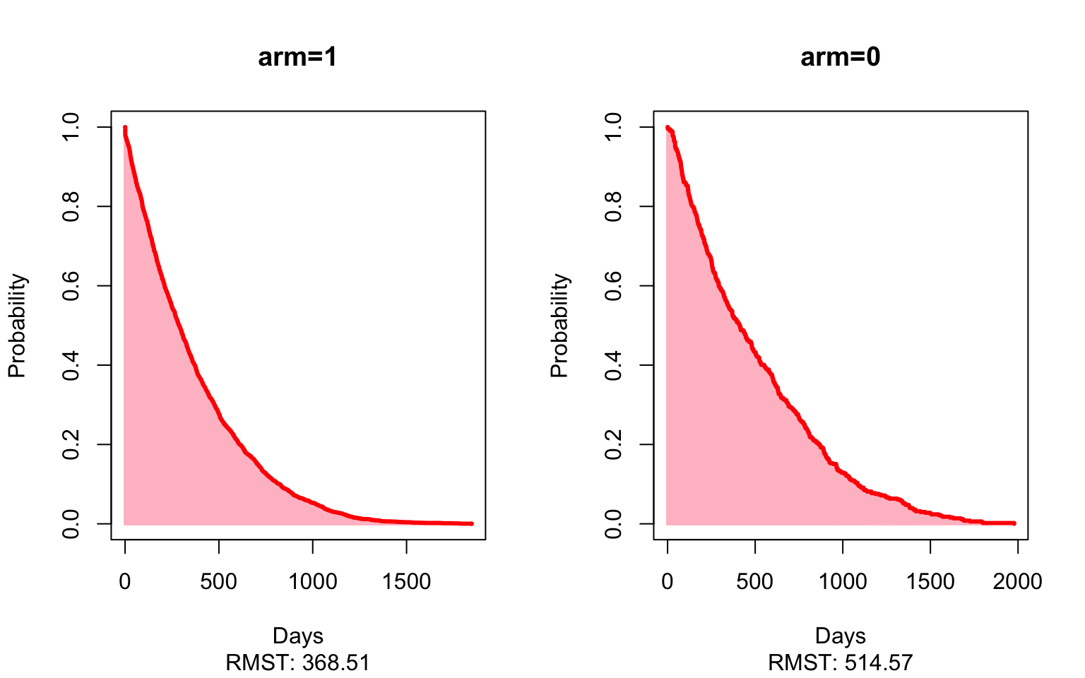
results## Est. lower .95 upper .95 p
## RMST (arm=1)-(arm=0) -146.0563345 -183.5178503 -108.5948186 2.145728e-14
## RMST (arm=1)/(arm=0) 0.7161582 0.6636577 0.7728118 8.358923e-18
## RMTL (arm=1)/(arm=0) 1.1114568 1.0804246 1.1433802 2.593745e-13Here, the matched estimate of -49 (-88, -9) shows that patients who receive an oral therapy first-line stopped treatment on average 49 days sooner than patients given the immunotherapy first-line, restricting to five years of follow-up. In other words, we’d expect patients who received an oral therapy first-line stop all treatment much sooner than patients who received immunotherapy as their first-line therapy. Again, looking at the matched estimates now comparing immunotherapy to chemotherapy, patients who received chemotherapy as first-line stopped all treatment an average of 167 (120, 214) days sooner than those patients who started on immunotherapy.
Time Varying Outcome: Opioid Usage Post Treatment
plot_data <-firstline_opioid %>%
  group_by(t,Brand) %>%
  summarise(mean = mean(monthtotal), std=sqrt(var(monthtotal)), n = n(),
            median = median(monthtotal), q1=quantile(monthtotal,.25),
            q3=quantile(monthtotal,.75)) %>%
  filter(t<=6)

plot_data$Treatment<-as.numeric(plot_data$Brand)
plot_data$Treatment<-factor(plot_data$Treatment,levels=c(1,2,3),labels = c("Immunotherapy","Chemotherapy","Oral Therapy"))
plot_data$provfac <-factor(as.numeric(plot_data$Brand),levels=c(1,2,3),labels=c("Sip","Doc","AE"))
plot_data$t <- plot_data$t*30

plot_all <-firstline_opioid %>%
  dplyr::select(t,Brand,monthtotal) %>%
  filter(t<=6)

plot_all$Treatment<-as.numeric(plot_all$Brand)
plot_all$Treatment<-factor(plot_all$Treatment,levels=c(1,2,3),labels = c("Immunotherapy","Chemotherapy","Oral Therapy"))
plot_all$provfac <-factor(as.numeric(plot_all$Brand),levels=c(1,2,3),labels=c("Sip","Doc","AE"))

plot_all$mean <-plot_all$monthtotal

#plot_data <-plot_data[plot_data$Brand!="DOC",]

p <-ggplot(plot_data,aes(x=t,y=mean,group=Treatment,color=Treatment,fill=Treatment,linetype=Treatment,weight=n,shape=Treatment,alpha=n))   +
geom_smooth(method = lm, formula = y ~ splines::bs(x, 3), se = FALSE,size=0.8,alpha=0.4)+ geom_point(size=4.5) + labs(color='Treatment',x='Days Since Start of First Focus Drug',y='Mean Opioids Prescribed (MME)') +
  scale_x_continuous(breaks = seq(0, 180, by = 30)) +theme_minimal()+
  scale_alpha_continuous(range = c(0.5, 1)) +
  theme(#plot.title = element_text(hjust = 0.9,size=16),
                           axis.ticks.y=element_blank(),
                         panel.grid.minor=element_blank(),
                         text = element_text(size=16))
png(filename="./PS_plot4.png",height = 520,width = 640)
ggpar(p,palette="nejm")
dev.off()## quartz_off_screen
## 2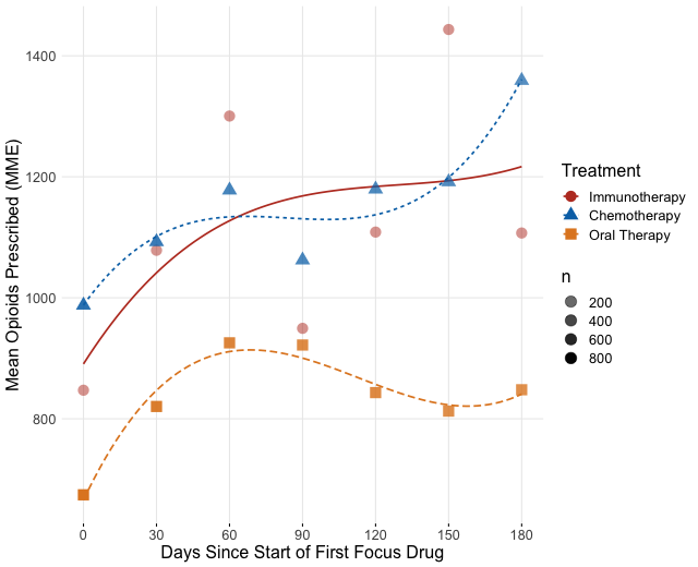
We can fit each of the methods in this outcome, adding covariates and smooths directly in the model, and fitting the model on a matched dataset. We use the R package mgcv. An important note when using IPTW and CBPS is that we are only weighting on the initial treatment, so at other time points the weights may bias the results. Also, we truncated the time to six months because many patients will only respond to or tolerate treatment for around six months before switching therapies to another focus treatment.
#these models take a long time to run, so output is saved
#then reloaded for illustration
#opioid data is stored in firstline_opioid dataset
#create ae to only compare oral therapy and immunotherapy
ae<-firstline_opioid[firstline_opioid$pae<=1,]
ae$treatment <-ae$pae
#select variables needed from ae
ae <-ae %>%
dplyr::select(Patid,monthtotal,t,treatment,pae,agecat,racecat,educat,
housecat,Division,
Product,met,Aso,diabetes,
hypertension,
CHF,osteoporosis,arrythmia,
uro)
#replace missings
ae$monthtotal <-ifelse(is.na(ae$monthtotal),0,ae$monthtotal)
ae$provfac<-factor(ae$pae,labels =c("Sip","AE"))
ae$Patid <-as.factor(ae$Patid)
ae$t <-as.integer(ae$t)
#keep only the first 6 periods
ae <-ae[ae$t<=6,]
modfullgroup <-bam(monthtotal~provfac +s(t,by=provfac,k=3)+s(Patid, bs="re",m=1),data=ae)
summary(modfullgroup)
p <- plot_diff(modfullgroup, view="t",
comp=list(provfac=c("AE", "Sip")),
cond=list(Condition=1),
ylim=c(-1000,2000),
xlim=c(0,6),
main="AE-Sip",
col=rainbow(6)[6],
rm.ranef=TRUE) #plot=FALSE
#optional plot of smoothed model difference over time
#plot_smooth(modfullgroup, view = "t",cond=list(provfac=c("Sip")),rm.ranef = TRUE, main="Model Dif",rug =FALSE)
#check which rows of plot data contain estimates at times of interest
p0 <-subset(p,t==0)
p0
#time we want may not be exeacly estimated, need something very close
#row 51 is what I took
p3 <-subset(p,t>2.8 & t<3.2)
p3
p6 <-subset(p,t>5.8 & t<6.2)
p6
#manual extraction of estimate and CI at desired time points
print(paste(p$est[c(1,51,100)],p$est[c(1,51,100)] - p$CI[c(1,51,100)],p$est[c(1,51,100)] + p$CI[c(1,51,100)]))
#now with covariate adjustments
modfullgroup2 <-bam(monthtotal~provfac +agecat+racecat+educat+
housecat+Division+
Product+met+Aso+diabetes+
hypertension+
CHF+osteoporosis+arrythmia+
uro + s(t,by=provfac,k=3) +
+ s(Patid, bs="re",m=1),
data=ae)
summary(modfullgroup2)
p <- plot_diff(modfullgroup2, view="t",
comp=list(provfac=c("AE", "Sip")),
cond=list(Condition=1),
ylim=c(-1000,2000),
main="AE-Sip",
col=rainbow(6)[6],
rm.ranef=TRUE)
print(paste(p$est[c(1,51,99)],p$est[c(1,51,99)] - p$CI[c(1,51,99)],p$est[c(1,51,99)] + p$CI[c(1,51,99)]))
#match based on start of focus drug treatment
ae_matching <-ae %>%
group_by(Patid) %>%
filter(row_number()==1)
ae_matching <-data.frame(ae_matching)
matched <- matchit(treatment~agecat+racecat+educat+housecat+Division+Product+met+Aso+diabetes+hypertension+CHF+osteoporosis+arrythmia+uro,data =ae_matching, method ="nearest",caliper=.2,ratio=4)
matched_sum<-summary(matched)
matched_sum$nn
matched_ae <- match.data(matched)
matched_ids <-unique(matched_ae$Patid)
#spline adjustment
m_ae <- ae %>%
filter(Patid %in% matched_ids)
matchedmodreg <-bam(monthtotal~provfac + s(t,by=provfac,k=3) +
s(Patid, bs="re",m=1),
data=m_ae)
summary(matchedmodreg)
p <- plot_diff(matchedmodreg, view="t",
comp=list(provfac=c("AE", "Sip")),
cond=list(Condition=1),
ylim=c(-1000,2000),
main="AE-Sip",
col=rainbow(6)[6],
rm.ranef=TRUE)
print(paste(p$est[c(1,51,99)],p$est[c(1,51,99)] - p$CI[c(1,51,99)],p$est[c(1,51,99)] + p$CI[c(1,51,99)]))
#Now IPTW based on first drug
propae <-glm(provfac~agecat+racecat+educat+housecat+Division+Product+met+Aso+diabetes+
hypertension+CHF+osteoporosis+arrythmia+uro,data=ae_matching,family=binomial(link='logit'))
ae_matching$pr_score <-predict(propae, type = "response")
summary(ae_matching$pr_score)
ae_matching$pr_score_trim <-ifelse(ae_matching$pr_score<.01,.01,ae_matching$pr_score)
ae_matching$pr_score_trim <-ifelse(ae_matching$pr_score>.99,.99,ae_matching$pr_score_trim)
ae_matching$IPTW <-ae_matching$treatment/ae_matching$pr_score_trim + (1-ae_matching$treatment)/(1-ae_matching$pr_score_trim)
cbps <-CBPS(treatment~agecat+racecat+educat+housecat+Division+Product+met+Aso+diabetes+
hypertension+CHF+osteoporosis+arrythmia+uro,data=ae_matching,standardize=TRUE,method="exact")
ae_matching$CBPS <-cbps$weights
#normalize weights for bam
ae_matching$st_weight <-ae_matching$IPTW / mean(ae_matching$IPTW)
ae_matching<-data.frame(ae_matching)
ae_matching <- ae_matching %>%
dplyr::select(Patid,pr_score,pr_score_trim,IPTW,CBPS,st_weight)
ae <-left_join(ae,ae_matching,by="Patid")
prep <-bam(monthtotal~provfac + s(t,by=provfac,k=3) + s(pr_score,k=4) +
s(Patid, bs="re",m=1),
data=ae)
summary(prep)
p <- plot_diff(prep, view="t",
comp=list(provfac=c("AE", "Sip")),
cond=list(Condition=1),
ylim=c(-1000,2000),
main="AE-Sip",
col=rainbow(6)[6],
rm.ranef=TRUE)
print(paste(p$est[c(1,51,99)],p$est[c(1,51,99)] - p$CI[c(1,51,99)],p$est[c(1,51,99)] + p$CI[c(1,51,99)]))
aeiptw <-bam(monthtotal~provfac + s(t,by=provfac,k=3) +
s(Patid, bs="re",m=1),
data=ae, weights = st_weight)
summary(aeiptw)
p <- plot_diff(aeiptw, view="t",
comp=list(provfac=c("AE", "Sip")),
cond=list(Condition=1),
ylim=c(-1000,2000),
main="AE-Sip",
col=rainbow(6)[6],
rm.ranef=TRUE)
print(paste(p$est[c(1,51,99)],p$est[c(1,51,99)] - p$CI[c(1,51,99)],p$est[c(1,51,99)] + p$CI[c(1,51,99)]))
aecbps <-bam(monthtotal~provfac + s(t,by=provfac,k=3) +
s(Patid, bs="re",m=1),
data=ae, weights = CBPS)
summary(aecbps)
p <- plot_diff(aecbps, view="t",
comp=list(provfac=c("AE", "Sip")),
cond=list(Condition=1),
ylim=c(-1000,2000),
main="AE-Sip",
col=rainbow(6)[6],
rm.ranef=TRUE)
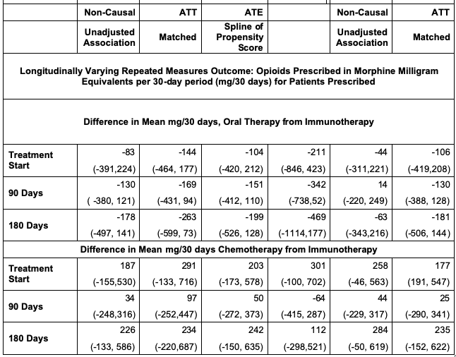
print(paste(p$est[c(1,51,99)],p$est[c(1,51,99)] - p$CI[c(1,51,99)],p$est[c(1,51,99)] + p$CI[c(1,51,99)])) The spline adjusted estimate for the difference in mean daily opioid prescribed 90 days after treatment start is -151 (-412, 110) MME. This suggests that on average, of those given opioids, patients starting with immunotherapy may be prescribed less opioids than those starting with oral therapy 90 days after treatment start. The confidence interval is noticeably wide. The IPTW estimate at this same time point is even less certain with -342 (-738,52).
All Tabled Results
Sensitivity Analysis
We assessed robustness of ATE estimates by looking at the vibration of effects to many propensity score models based on observed set of confounders, and also calculating an E-value for unobserved confounding. For the binary outcome, we assessed the estimates to all possible propensity score models for three selected methods. Age was included as a baseline predictor in all models. E-values were calculated for the model that included the full covariate set. The below figure shows the results of these analyses. The figure shows that we cannot detect a meaningful difference between the immunotherapy and oral therapy with either of these outcomes across an ensemble of propensity score models. However, we see with the chemotherapy comparisons that all estimates are significant across most choices of the propensity model. Yet, the E-values of 3.1, 3.05, and 3.17 indicate that results can be explained away by a modest unobserved confounder, so we should be cautious generalizing these results.
covariates <- ~ racecat+educat+housecat+Division+Product+met+Aso+diabetes+hypertension+CHF+osteoporosis+arrythmia+uro

base_ps_model <- treatment~agecat
base_out_model <- er60~treatment
base_out_spline <- er60~treatment+bs(pr_score)


vib_oral_spline <- conductVibration_ps(base_out_spline, base_out_model,oral60, covariates, family='binomial')

vib_oral_iptw <- conductVibration_ps(base_ps_model, base_out_model,oral60, covariates, family='binomial')


oral_spline <-plot_vibration_cox(vib_oral_spline,type='contour', alpha=.3)

oral_iptw <-plot_vibration_cox(vib_oral_iptw,type='contour', alpha=.3)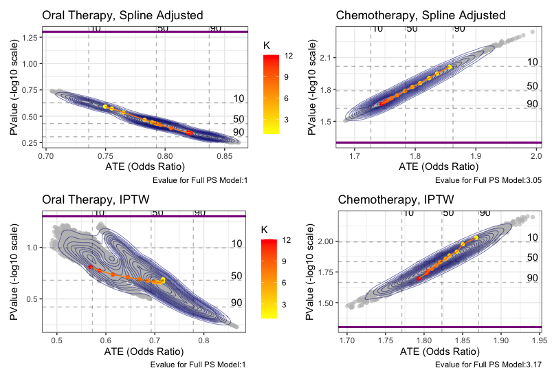
Conclusion
In summary, the methods shown here outline a standard process for conducting comparative effectiveness research in claims databases. It is important to note that these tools cannot perfectly answer comparative effectiveness questions, even with the most extensive data. Careful consideration is required by the researchers as to what variables are confounding treatment and outcome, and what method and assumptions best fit the study. Adding sensitivity analysis to a study can add understanding to the robustness and generalizations of the results. We hope the extensive detail, documentation, and accompanying code aide researchers in their own studies and improve replication among these studies. See paper for more discussion
References
Ali, M. Sanni, Rolf H.H. Groenwold, Svetlana V. Belitser, Wiebe R. Pestman, Arno W. Hoes, Kit C.B. Roes, Anthonius de Boer, and Olaf H. Klungel. 2015. “Reporting of Covariate Selection and Balance Assessment in Propensity Score Analysis Is Suboptimal: A Systematic Review.” Journal of Clinical Epidemiology 68 (2): 122–31. https://doi.org/10.1016/J.JCLINEPI.2014.08.011.
Andersen, Robert.: Modern Methods for Robust Regression 1–6. (2019)
Andersen PK, Perme MP. Pseudo-observations in survival analysis. Stat Methods Med Res. 2010;19(1):71-99. doi:10.1177/0962280209105020
Austin, Peter C. 2008a. “A Critical Appraisal of Propensity-Score Matching in the Medical Literature between 1996 and 2003.” Statistics in Medicine 27 (12): 2037–49. https://doi.org/10.1002/sim.3150.
Austin, Peter C. 2009a. “Balance Diagnostics for Comparing the Distribution of Baseline Covariates between Treatment Groups in Propensity-Score Matched Samples.” Statistics in Medicine 28 (25): 3083–3107. https://doi.org/10.1002/sim.3697.
Austin, Peter C. 2009b. “The Relative Ability of Different Propensity Score Methods to Balance Measured Covariates Between Treated and Untreated Subjects in Observational Studies.” Edited by Kathryn M. McDonald. Medical Decision Making 29 (6): 661–77. https://doi.org/10.1177/0272989X09341755.
Austin, Peter C. 2011a. “Optimal Caliper Widths for Propensity‐ score Matching When Estimating Differences in Means and Differences in Proportions in Observational Studies.” Pharmaceutical Statistics 10 (2): 150–61. https://doi.org/10.1002/PST.433.
Austin, Peter C., Paul Grootendorst, and Geoffrey M. Anderson. 2007. “A Comparison of the Ability of Different Propensity Score Models to Balance Measured Variables between Treated and Untreated Subjects: A Monte Carlo Study.” Statistics in Medicine 26 (4): 734– 53. https://doi.org/10.1002/sim.2580.
Austin, P.C. (2008b), Assessing balance in measured baseline covariates when using many‐to‐one matching on the propensity‐score. Pharmacoepidem. Drug Safe., 17: 1218-1225. doi:10.1002/pds.1674
Austin, Peter C. 2011b. “An Introduction to Propensity Score Methods for Reducing the Effects of Confounding in Observational Studies.” Multivariate Behavioral Research 46 (3): 399–424.https://doi.org/10.1080/00273171.2011.568786.
Austin, Peter C. 2018. “Assessing the Performance of the Generalized Propensity Score for Estimating the Effect of Quantitative or Continuous Exposures on Binary Outcomes.” Statistics in Medicine 37 (11): 1874–94. https://doi.org/10.1002/sim.7615.
Barocas, D.A. and Penson, D.F. (2010), Racial variation in the pattern and quality of care for prostate cancer in the USA: mind the gap. BJU International, 106: 322-328. doi:10.1111/j.1464-410X.2010.09467.x
Bates, Douglas, and William Venables. 2020 “Splines Package | R Documentation.” Accessed April 25, 2020. https://www.rdocumentation.org/packages/splines/versions/3.6.2.
Berger, Marc L., Harold Sox, Richard J. Willke, Diana L. Brixner, Hans-Georg Eichler, Wim Goettsch, David Madigan, et al. 2017. “Good Practices for Real-World Data Studies of Treatment and/or Comparative Effectiveness: Recommendations from the Joint ISPOR- ISPE Special Task Force on Real-World Evidence in Health Care Decision Making.” Pharmacoepidemiology and Drug Safety 26 (9): 1033–39. https://doi.org/10.1002/pds.4297.
Birnbaum, Howard G., Pierre Y. Cremieux, Paul E. Greenberg, Jacques LeLorier, JoAnn Ostrander, and Laura Venditti. 1999. “Using Healthcare Claims Data for Outcomes Research and Pharmacoeconomic Analyses.” PharmacoEconomics 16 (1): 1–8. https://doi.org/10.2165/00019053-199916010-00001.
Braitman, Leonard E., and Paul R. Rosenbaum. 2002. “Rare Outcomes, Common Treatments: Analytic Strategies Using Propensity Scores.” Annals of Internal Medicine. American College of Physicians. https://doi.org/10.7326/0003-4819-137-8-200210150-00015.
Brookhart, M. Alan, Sebastian Schneeweiss, Kenneth J. Rothman, Robert J. Glynn, Jerry Avorn, and Til Stürmer. 2006. “Variable Selection for Propensity Score Models.” American Journal of Epidemiology 163 (12): 1149–56. https://doi.org/10.1093/aje/kwj149.
Brookhart, M Alan, Richard Wyss, J Bradley Layton, and Til Stürmer. 2013. “Propensity Score Methods for Confounding Control in Nonexperimental Research.” Circulation. Cardiovascular Quality and Outcomes 6 (5): 604–11. https://doi.org/10.1161/CIRCOUTCOMES.113.000359.
Caram, Megan E. V., Shikun Wang, Phoebe Tsao, Jennifer J. Griggs, David C. Miller, Brent K. Hollenbeck, Paul Lin, and Bhramar Mukherjee. 2019a. “Patient and Provider Variables Associated with Systemic Treatment of Advanced Prostate Cancer.” Urology Practice 6 (4): 234–42. https://doi.org/10.1097/UPJ.0000000000000020.
Caram, Megan E.V., Ryan Ross, Paul Lin, and Bhramar Mukherjee. 2019b. “Factors Associated with Use of Sipuleucel-T to Treat Patients With Advanced Prostate Cancer.” JAMA Network Open 2 (4): e192589. https://doi.org/10.1001/jamanetworkopen.2019.2589.
CDC. n.d. “Data Resources | Drug Overdose.” Accessed April 25, 2020a. https://www.cdc.gov/drugoverdose/resources/data.html.
CMS. n.d. “Measure Methodology.” Accessed April 25, 2020b. https://www.cms.gov/Medicare/Quality-Initiatives-Patient-Assessment- Instruments/HospitalQualityInits/Measure-Methodology.
Cole, S. R., and M. A. Hernan. 2008. “Constructing Inverse Probability Weights for Marginal Structural Models.” American Journal of Epidemiology 168 (6): 656–64. https://doi.org/10.1093/aje/kwn164.
Conner, Sarah C., Lisa M. Sullivan, Emelia J. Benjamin, Michael P. LaValley, Sandro Galea, and Ludovic Trinquart. 2019. “Adjusted Restricted Mean Survival Times in Observational Studies.” Statistics in Medicine 38 (20): 3832–60. https://doi.org/10.1002/sim.8206.
D'Agostino, R., Lang, W., Walkup, M. et al. Examining the Impact of Missing Data on Propensity Score Estimation in Determining the Effectiveness of Self-Monitoring of Blood Glucose (SMBG). Health Services & Outcomes Research Methodology 2, 291–315 (2001). https://doi.org/10.1023/A:1020375413191
D’Agostino Jr, R.B. & Rubin, Donald. (2000). Estimating and Using Propensity Scores with Partially Missing Data. Journal of the American Statistical Association. 95. 749-759. doi: 10.2307/2669455.
D'Ascenzo F, Cavallero E, Biondi-Zoccai G, et al. Use and Misuse of Multivariable Approaches in Interventional Cardiology Studies on Drug-Eluting Stents: A Systematic Review. J Interv Cardiol. 2012;25(6):611-621. doi:10.1111/j.1540-8183.2012.00753.x
Deb, Saswata, Peter C. Austin, Jack V. Tu, Dennis T. Ko, C. David Mazer, Alex Kiss, and Stephen E. Fremes. 2016. “A Review of Propensity-Score Methods and Their Use in Cardiovascular Research.” Canadian Journal of Cardiology 32 (2): 259–65. https://doi.org/10.1016/J.CJCA.2015.05.015.
Desai, Rishi J., Ameet Sarpatwari, Sara Dejene, Nazleen F. Khan, Joyce Lii, James R. Rogers, Sarah K. Dutcher, et al. 2019. “Comparative Effectiveness of Generic and Brand-Name Medication Use: A Database Study of Us Health Insurance Claims.” PLoS Medicine 16 (3). https://doi.org/10.1371/journal.pmed.1002763.
Dickstein, Craig, and Renu Gehring. 2014. Administrative Healthcare Data A Guide to Its Origin, Content, and Application Using SAS ®. SAS Institute. Elixhauser, Anne, Claudia Steiner, D. Robert Harris, and Rosanna M. Coffey. 1998. “Comorbidity Measures for Use with Administrative Data.” Medical Care 36 (1): 8–27. https://doi.org/10.1097/00005650-199801000-00004.
FDA. 2011. “Best Practices for Conducting and Reporting Pharmacoepidemiologic Safety Studies Using Electronic Healthcare Data Sets.”
FDA. 2018. “Framework for FDA’s Real-World Evidence Program.” Garrido, M.M., Kelley, A.S., Paris, J., Roza, K., Meier, D.E., Morrison, R.S. and Aldridge, M.D. (2014), Methods for Constructing and Assessing Propensity Scores. Health Serv Res, 49: 1701-1720. https://doi.org/10.1111/1475-6773.12182
Grimes, David A. 2010. “Epidemiologic Research Using Administrative Databases.” Obstetrics & Gynecology 116 (5): 1018–19. https://doi.org/10.1097/AOG.0b013e3181f98300.
HCUP. n.d. “Clinical Classifications Software (CCS) for ICD-10-PCS (Beta Version).” Accessed April 25, 2020. https://www.hcup-us.ahrq.gov/toolssoftware/ccs10/ccs10.jsp.
Hernán, Miguel A., and James M. Robins. 2016. “Using Big Data to Emulate a Target Trial When a Randomized Trial Is Not Available.” American Journal of Epidemiology 183 (8): 758–64. https://doi.org/10.1093/aje/kwv254.
Hirano, Keisuke, and Guido W. Imbens. 2005. “The Propensity Score with Continuous Treatments.” In Applied Bayesian Modeling and Causal Inference from Incomplete-Data Perspectives: An Essential Journey with Donald Rubin’s Statistical Family, 73–84. Wiley Blackwell. https://doi.org/10.1002/0470090456.ch7.
Ho, Daniel, Kosuke Imai, Gary King, and Elizabeth Stuart. 2018. “Package ‘MatchIt’ Title Nonparametric Preprocessing for Parametric Causal Inference.” https://doi.org/10.1093/pan/mpl013.
Hoffman RM, Gilliland FD, Eley JW, et al. Racial and ethnic differences in advanced-stage prostate cancer: the Prostate Cancer Outcomes Study. J Natl Cancer Inst. 2001;93(5):388-395. https://doi.org/10.1093/jnci/93.5.388
Hoover, Karen W., Guoyu Tao, Charlotte K. Kent, and Sevgi O. Aral. 2011. “Epidemiologic Research Using Administrative Databases: Garbage In, Garbage Out.” Obstetrics & Gynecology 117 (3): 729. https://doi.org/10.1097/AOG.0b013e31820cd18a.
Imai, K. and Ratkovic, M. (2014), Covariate balancing propensity score. J. R. Stat. Soc. B, 76: 243-263. https://doi.org/10.1111/rssb.12027
Imbens, Guido. (2004). Nonparametric Estimation of Average Treatment Effects Under Exogeneity: A Review. The Review of Economics and Statistics. 86. 4-29. https://doi.org/10.1162/003465304323023651.
Izurieta, Hector S., Xiyuan Wu, Yun Lu, Yoganand Chillarige, Michael Wernecke, Arnstein Lindaas, Douglas Pratt, et al. 2019. “Zostavax Vaccine Effectiveness among US Elderly Using Real-World Evidence: Addressing Unmeasured Confounders by Using Multiple Imputation after Linking Beneficiary Surveys with Medicare Claims.” Pharmacoepidemiology and Drug Safety 28 (7): 993–1001. https://doi.org/10.1002/pds.4801.
Jackevicius, Cynthia A, Jack V Tu, Harlan M Krumholz, Peter C Austin, Joseph S Ross, Therese A Stukel, Maria Koh, Alice Chong, and Dennis T Ko. 2016. “Comparative Effectiveness of Generic Atorvastatin and Lipitor® in Patients Hospitalized with an Acute Coronary Syndrome.” Journal of the American Heart Association 5 (4): e003350. https://doi.org/10.1161/JAHA.116.003350.
Joffe, Marshall M, Thomas R Ten Have, Harold I Feldman, and Stephen E Kimmel. 2004. “Model Selection, Confounder Control, and Marginal Structural Models.” The American Statistician 58 (4): 272–79. https://doi.org/10.1198/000313004X5824.
Johnson, Michael L., William Crown, Bradley C. Martin, Colin R. Dormuth, and Uwe Siebert. 2009. “Good Research Practices for Comparative Effectiveness Research: Analytic Methods to Improve Causal Inference from Nonrandomized Studies of Treatment Effects Using Secondary Data Sources: The ISPOR Good Research Practices for Retrospective Database Analysis Task Force Report—Part III.” Value in Health 12 (8): 1062–73. https://doi.org/10.1111/J.1524-4733.2009.00602.X.
Lee, Brian K., Justin Lessler, and Elizabeth A. Stuart. 2011. “Weight Trimming and Propensity Score Weighting.” Edited by Giuseppe Biondi-Zoccai. PLoS ONE 6 (3): e18174. https://doi.org/10.1371/journal.pone.0018174.
Lee, Brian K, Justin Lessler, and Elizabeth A Stuart. 2010. “Improving Propensity Score Weighting Using Machine Learning.” Statistics in Medicine 29 (3): 337–46. https://doi.org/10.1002/sim.3782.
Li, Fan, Kari Lock Morgan, and Alan M. Zaslavsky. 2018. “Balancing Covariates via Propensity Score Weighting.” Journal of the American Statistical Association 113 (521): 390–400. https://doi.org/10.1080/01621459.2016.1260466. Lumley, Thomas. 2020. R package “Survey” https://cran.r-project.org/web/packages/survey/index.html
Lunceford, Jared K, and Marie Davidian. 2017. “Stratification and Weighting Via the Propensity Score in Estimation of Causal Treatment Effects: A Comparative Study.”
Morgan, Stephen L., and Jennifer J. Todd. 2008. “6. A Diagnostic Routine for the Detection of Consequential Heterogeneity of Causal Effects.” Sociological Methodology 38 (1): 231–82. https://doi.org/10.1111/j.1467-9531.2008.00204.x.
Motheral, Brenda, John Brooks, Mary Ann Clark, William H. Crown, Peter Davey, Dave Hutchins, Bradley C. Martin, and Paul Stang. 2003. “A Checklist for Retrospective Database Studies—Report of the ISPOR Task Force on Retrospective Databases.” Value in Health 6 (2): 90–97. https://doi.org/10.1046/J.1524-4733.2003.00242.X.
Nidey, Nichole, Ryan Carnahan, Knute D. Carter, Lane Strathearn, Wei Bao, Andrea Greiner, Laura Jelliffee-Pawlowski, Karen M. Tabb, and Kelli Ryckman. 2020. “Association of Mood and Anxiety Disorders and Opioid Prescription Patterns Among Postpartum Women.” The American Journal on Addictions, April. https://doi.org/10.1111/ajad.13028.
Noe, Megan H., Daniel B. Shin, Jalpa A. Doshi, David J. Margolis, and Joel M. Gelfand. 2019. “Prescribing Patterns Associated With Biologic Therapies for Psoriasis from a United States Medical Records Database.” Journal of Drugs in Dermatology : JDD 18 (8): 745–50.
Normand, Sharon-Lise T., Mary Beth Landrum, Edward Guadagnoli, John Z. Ayanian, Thomas J. Ryan, Paul D. Cleary, and Barbara J. McNeil. 2001. “Validating Recommendations for Coronary Angiography Following Acute Myocardial Infarction in the Elderly: A Matched Analysis Using Propensity Scores.” Journal of Clinical Epidemiology 54 (4): 387–98. https://doi.org/10.1016/S0895-4356(00)00321-8.
O’Neal, Wesley T., Pratik B. Sandesara, J’Neka S. Claxton, Richard F. MacLehose, Lin Y. Chen, Lindsay G. S. Bengtson, Alanna M. Chamberlain, Faye L. Norby, Pamela L. Lutsey, and Alvaro Alonso. 2018. “Provider Specialty, Anticoagulation Prescription Patterns, and Stroke Risk in Atrial Fibrillation.” Journal of the American Heart Association 7 (6). https://doi.org/10.1161/JAHA.117.007943.
Patel, Chirag J., Belinda Burford, and John P.A. Ioannidis. 2015. “Assessment of Vibration of Effects Due to Model Specification Can Demonstrate the Instability of Observational Associations.” Journal of Clinical Epidemiology 68 (9): 1046–58. https://doi.org/10.1016/j.jclinepi.2015.05.029.
Perkins, Susan M., Wanzhu Tu, Michael G. Underhill, Xiao-Hua Zhou, and Michael D. Murray. 2000. “The Use of Propensity Scores in Pharmacoepidemiologic Research.” Pharmacoepidemiology and Drug Safety 9 (2): 93–101. https://doi.org/10.1002/(SICI)1099- 1557(200003/04)9:2<93::AID-PDS474>3.0.CO;2-I.
Robins, James. 1986. “A New Approach to Causal Inference in Mortality Studies with a Sustained Exposure Period-Application to Control of the Healthy Worker Survivor Effect.” Mathematical Modelling 7 (9–12): 1393–1512. https://doi.org/10.1016/0270- 0255(86)90088-6.
Rosenbaum, P R, and D B Rubin. 1985a. “The Bias Due to Incomplete Matching.” Biometrics 41 (1): 103–16. https://doi.org/10.2307/2530647.
Rosenbaum, Paul R. 1987. “Model-Based Direct Adjustment.” Journal of the American Statistical Association 82 (398): 387–94. https://doi.org/10.1080/01621459.1987.10478441.
Rosenbaum, Paul R., and Donald B. Rubin. 1984. “Reducing Bias in Observational Studies Using Subclassification on the Propensity Score.” Journal of the American Statistical Association 79 (387): 516. https://doi.org/10.2307/2288398.
Rosenbaum, Paul R. 1985b. “Constructing a Control Group Using Multivariate Matched Sampling Methods That Incorporate the Propensity Score.” The American Statistician 39 (1): 33. https://doi.org/10.2307/2683903.
Rosenbaum, Paul R, and Donald B Rubin. 1983. “The Central Role of the Propensity Score in Observational Studies for Causal Effects.” Biometrika. Vol. 70.
Royston, P., Parmar, M.K. Restricted mean survival time: an alternative to the hazard ratio for the design and analysis of randomized trials with a time-to-event outcome. BMC Med Res Methodol 13, 152 (2013). https://doi.org/10.1186/1471-2288-13-152
Rubin, Donald B. 1974. “Estimating Causal Effects of Treatments in Randomized And Nonrandomized Studies 1.” Journal of Educational Psychology. Vol. 66. Rubin, Donald B. 2005. “Causal Inference Using Potential Outcomes: Design, Modeling, Decisions.” https://doi.org/10.1198/016214504000001880.
Rubin, Donald B, and Neal Thomas. 1996. “Matching Using Estimated Propensity Scores: Relating Theory to Practice.” Vol. 52. Schneeweiss, Sebastian, and Jerry Avorn. 2005. “A Review of Uses of Health Care Utilization Databases for Epidemiologic Research on Therapeutics.” Journal of Clinical Epidemiology 58 (4): 323–37. https://doi.org/10.1016/j.jclinepi.2004.10.012.
Setoguchi, Soko, Sebastian Schneeweiss, M. Alan Brookhart, Robert J. Glynn, and E. Francis Cook. 2008. “Evaluating Uses of Data Mining Techniques in Propensity Score Estimation: A Simulation Study.” Pharmacoepidemiology and Drug Safety 17 (6): 546–55. https://doi.org/10.1002/pds.1555.
Sherman, Rachel E., Steven A. Anderson, Gerald J. Dal Pan, Gerry W. Gray, Thomas Gross, Nina L. Hunter, Lisa LaVange, et al. 2016. “Real-World Evidence — What Is It and What Can It Tell Us?” New England Journal of Medicine 375 (23): 2293–97. https://doi.org/10.1056/NEJMsb1609216.
Shi, Xu, Robert Wellman, Patrick J. Heagerty, Jennifer C. Nelson, and Andrea J. Cook. 2020. “Safety Surveillance and the Estimation of Risk in Select Populations: Flexible Methods to Control for Confounding While Targeting Marginal Comparisons via Standardization.” Statistics in Medicine 39 (4): 369–86. https://doi.org/10.1002/sim.8410.
Snowden, Jonathan, Sherri Rose, and Kathleen Mortimer. 2011. “Implementation of G- Computation on a Simulated Data Set: Demonstration of a Causal Inference Technique.” American Journal of Epidemiology. 2011. https://academic.oup.com/aje/article/173/7/731/104142.
Stefanski, Leonard A., and Dennis D. Boos. “The Calculus of M-Estimation.” The American Statistician, vol. 56, no. 1, 2002, pp. 29–38. JSTOR, https://doi.org/10.1198/000313002753631330
Stuart, Elizabeth A. 2010. “Matching Methods for Causal Inference: A Review and a Look Forward.” Statistical Science : A Review Journal of the Institute of Mathematical Statistics 25 (1): 1–21. https://doi.org/10.1214/09-STS313.
Stuart, Elizabeth A, Eva DuGoff, Michael Abrams, David Salkever, and Donald Steinwachs. 2013. “Estimating Causal Effects in Observational Studies Using Electronic Health Data: Challenges and (Some) Solutions.” EGEMS (Washington, DC) 1 (3): 1038. https://doi.org/10.13063/2327-9214.1038.
Susanti, Yuliana, Hasih Pratiwi, Sri H Sulistijowati, and Twenty Liana. 2014. “P A M Estimation, S Estimation, And Mm Estimation in Robust Regression.” International Journal of Pure and Applied Mathematics 91 (3): 349–60. https://doi.org/10.12732/ijpam.v91i3.7.
Tian, Lu, Lihui Zhao, and L. J. Wei. 2014. “Predicting the Restricted Mean Event Time with the Subject’s Baseline Covariates in Survival Analysis.” Biostatistics 15 (2): 222–33. https://doi.org/10.1093/biostatistics/kxt050.
Tyree, Patrick T, Bonnie K Lind, and William E Lafferty. 2006. “Challenges of Using Medical Insurance Claims Data for Utilization Analysis.” American Journal of Medical Quality : The Official Journal of the American College of Medical Quality 21 (4): 269–75. https://doi.org/10.1177/1062860606288774.
Uno, Hajime, Brian Claggett, Lu Tian, Eisuke Inoue, Paul Gallo, Toshio Miyata, Deborah Schrag, et al. 2014. “Moving beyond the Hazard Ratio in Quantifying the Between-Group Difference in Survival Analysis.” Journal of Clinical Oncology 32 (22): 2380–85. https://doi.org/10.1200/JCO.2014.55.2208.
VanderWeele, Tyler J. 2019. “Principles of Confounder Selection.” European Journal of Epidemiology 34 (3). https://doi.org/10.1007/s10654-019-00494-6.
Venkatesh, Arjun K., Hao Mei, Keith E. Kocher, Michael Granovsky, Ziad Obermeyer, Erica S. Spatz, Craig Rothenberg, Harlan M. Krumholz, and Zhenqui Lin. 2017. “Identification of Emergency Department Visits in Medicare Administrative Claims: Approaches and Implications.” Academic Emergency Medicine 24 (4): 422–31. https://doi.org/10.1111/acem.13140.
von Elm, Erik; Altman, Douglas G.; Egger, Matthias; Pocock, Stuart J.; Gøtzsche, Peter C.; Vandenbroucke, Jan P.∥ The Strengthening the Reporting of Observational Studies in Epidemiology (STROBE) Statement: Guidelines for Reporting Observational Studies, Epidemiology: November 2007 - Volume 18 - Issue 6 - p 800-804 doi: 10.1097/EDE.0b013e31815776
Ward, E., Jemal, A., Cokkinides, V., Singh, G.K., Cardinez, C., Ghafoor, A. and Thun, M. (2004), Cancer Disparities by Race/Ethnicity and Socioeconomic Status. CA: A Cancer Journal for Clinicians, 54: 78-93. doi:10.3322/canjclin.54.2.78
Weele, Tyler J. Van Der, and Peng Ding. 2017. “Sensitivity Analysis in Observational Research: Introducing the E-Value.” Annals of Internal Medicine 167 (4): 268–74. https://doi.org/10.7326/M16-2607.
Weitzen, Sherry, Kate L. Lapane, Alicia Y. Toledano, Anne L. Hume, and Vincent Mor. 2004. “Principles for Modeling Propensity Scores in Medical Research: A Systematic Literature Review.” Pharmacoepidemiology and Drug Safety 13 (12): 841–53. https://doi.org/10.1002/pds.969.
Westreich, Daniel, Justin Lessler, and Michele Jonsson Funk. 2010. “Propensity Score Estimation: Neural Networks, Support Vector Machines, Decision Trees (CART), and Meta-Classifiers as Alternatives to Logistic Regression.” Journal of Clinical Epidemiology 63 (8): 826–33. https://doi.org/10.1016/J.JCLINEPI.2009.11.020.
Wilson, John, and Adam Bock. 2012. “Optum The Benefit of Using Both Claims Data and Electronic Medical Record Data in Health Care Analysis White Paper.”
Wood, Simon, Natalya Pya, and Benjamin Safken. 2018. “Package ‘mgcv’ Title Mixed GAM Computation Vehicle with Automatic Smoothness Estimation.”
Wyss, Richard, Alan R. Ellis, M. Alan Brookhart, Cynthia J. Girman, Michele Jonsson Funk, Robert LoCasale, and Til Stürmer. 2014. “The Role of Prediction Modeling in Propensity Score Estimation: An Evaluation of Logistic Regression, BCART, and the Covariate- Balancing Propensity Score.” American Journal of Epidemiology 180 (6): 645–55. https://doi.org/10.1093/aje/kwu181.
Wyss, Richard, Cynthia J Girman, Robert J LoCasale, Alan M Brookhart, and Til Stürmer. 2013. “Variable Selection for Propensity Score Models When Estimating Treatment Effects on Multiple Outcomes: A Simulation Study.” Pharmacoepidemiology and Drug Safety 22 (1): 77–85. https://doi.org/10.1002/pds.3356.
Yao, Xiaoxin I., Xiaofei Wang, Paul J. Speicher, E. Shelley Hwang, Perry Cheng, David H. Harpole, Mark F. Berry, Deborah Schrag, and Herbert H. Pang. 2017. “Reporting and Guidelines in Propensity Score Analysis: A Systematic Review of Cancer and Cancer Surgical Studies.” JNCI: Journal of the National Cancer Institute 109 (8). https://doi.org/10.1093/jnci/djw323.
Yu, Bin, and Karl Kumbier. 2020. “Veridical Data Science.” Proceedings of the National Academy of Sciences 117 (8): 201901326. https://doi.org/10.1073/pnas.1901326117.